Which examples are still missing from the prompt?

Jiayi Xin

Topics: Large language models · In-context learning · Coverage estimation

Using unseen-cluster estimation to improve in-context demonstration selection

Why demonstration selection matters

In-context learning (ICL) lets a language model perform a task by conditioning on examples placed directly in its prompt. Each demonstration pairs an input with its desired output. We concatenate these examples with a new input and let the model predict its output, keeping the model’s parameters fixed.

For an illustrative banking-intent task, the prompt could be:

Identify the intent of each message.

Message: My card still hasn’t arrived. Intent: card delivery

Message: The same purchase appears twice. Intent: duplicate charge

Message: When will my card be delivered? Intent:

The intended answer is “card delivery.” The examples specify the task and output format without a parameter update.

Prior studies show that ICL performance can vary substantially with the selected demonstrations, even at a fixed budget (Su et al., 2022; Peng et al., 2024). Peng et al. also show that the best demonstrations can differ across inference models. This motivates our central question: which examples should we combine to make the most of a limited prompt budget?

Choosing from a large candidate pool

One motivating application starts with a large unlabelled dataset of task inputs and a limited annotation budget: choose useful inputs, obtain their labels, and use the resulting input–output pairs as demonstrations. UCS constructs its clusters and coverage statistics from inputs alone. Our experiments use an already-labelled candidate pool and usually limit each prompt to ten demonstrations. This is a prompt-size budget; query-dependent selection can use different labelled examples for different test inputs.

With that budget fixed, we focus on the composition of the whole set. Several individually relevant examples may represent similar patterns, leaving other task-relevant patterns absent.

In Unseen Coverage Selection (UCS), we take a knowledge-based view of demonstration selection: which task-relevant concepts and skills does the prompt expose, and which are still missing? Similarity, diversity, and information-theoretic objectives capture useful aspects of a demonstration set. Our motivation in Figure 1 is to add knowledge coverage as a complementary, set-level criterion.

To make this question measurable, we use representation-derived clusters as countable proxies for task knowledge. We define the clusters over the candidate pool, then count how often each appears in a proposed demonstration set. Here, unseen means absent from that selected set. We estimate how many additional clusters further sampling from the same pool would reveal and use this estimate to guide selection.

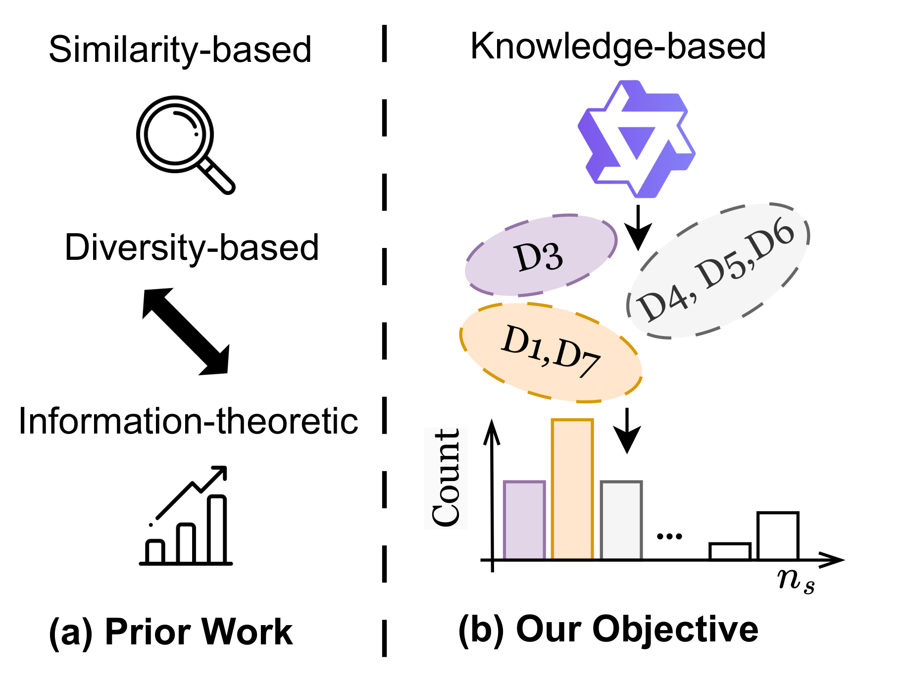
UCS models knowledge coverage through the latent clusters represented by a demonstration set. Their frequencies connect the selected examples to the question of what remains unseen.

Turning examples into countable patterns

To estimate unseen clusters, we first need to define a cluster. UCS embeds the input of each demonstration using the same language model that will answer the test queries. Mean pooling over non-padding tokens produces one vector per input; demonstration labels are excluded.

We then learn a dictionary that approximates each embedding as a weighted combination of shared components, or atoms. The weights form a code vector. We normalize these vectors and cluster them with DBSCAN using cosine distance. This groups examples with similar combinations of atoms, retaining distinctions that assignment to a single dominant atom would discard. In the clustering procedure, each DBSCAN noise point receives its own singleton cluster. This preprocessing requires fitting the dictionary and cluster assignments, while the language model remains frozen and no selection policy is trained.

The resulting clusters vary greatly in size. Figure 3 shows this long-tailed structure across three intent-classification datasets: many demonstrations occupy small or singleton clusters, while a few much larger clusters recur frequently. The colors also show that the distribution changes with the backbone model. This makes coverage both uneven and model-specific; repeatedly selecting from a dominant cluster can leave many less common patterns out of the prompt.

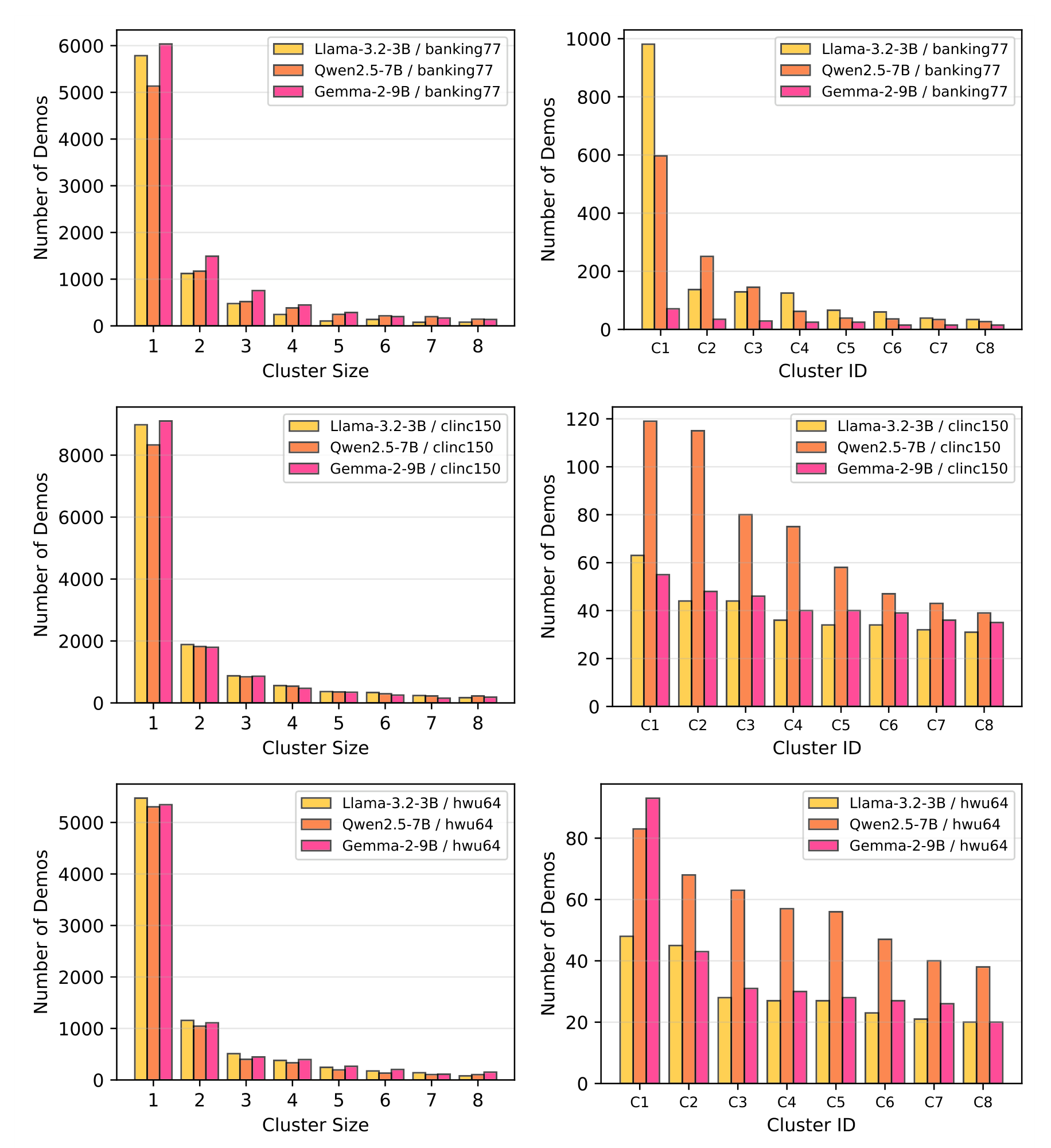
Rows show BANKING77, CLINC150, and HWU64. The left column counts demonstrations in clusters of size 1–8; the right shows the sizes of the eight largest clusters. Together they reveal the long tail that motivates looking beyond repeatedly sampled patterns.

Estimating the clusters still unseen

The statistical idea comes from estimating unseen species. A sample containing many types observed only once suggests that more types remain undiscovered. Repeated observations reveal how often sampling returns to familiar types. UCS combines these frequencies in a stabilized unseen-count estimator that we call Smoothed Good–Turing (SGT) in our paper. Its alternating-series form follows smoothed Good–Toulmin estimation, which predicts how many new types additional sampling would reveal.

For a candidate demonstration set $S$, let $n_u(S)$ count its examples from cluster $u$. The frequency spectrum records how many clusters appear exactly $s$ times:

Thus $f_1$ counts clusters represented once, $f_2$ counts those represented twice, and so on. Two sets can cover the same number of clusters yet have different repetition patterns, which this spectrum preserves.

Extrapolating further can amplify noise in these counts. The smoothing in UCS limits the influence of unstable higher-order terms, using damping and truncation to keep a few observations from dominating the estimate:

Here $t=m/\lvert S\rvert$ sets the horizon of $m$ additional draws from the same candidate-pool sampling process. The cutoff $M$ truncates the sum, and the weights $w_s(t,\alpha)\in[0,1]$ damp higher-order terms. The offset parameter $\alpha$ controls this damping. We use $t=5$, $M=20$, and $\alpha=1$ by default, and set negative or non-finite estimates to zero.

Let $K_{\mathrm{seen}}(S)$ be the number of distinct clusters represented in $S$. The coverage score adds the estimated number of new clusters to this observed count:

A high score favors both broad observed coverage and a frequency pattern suggesting further discoveries. We use this extrapolated count as a prior for ranking candidate sets and evaluate its usefulness through downstream ICL accuracy. We give the estimator and selection objective in Sections 3.5–3.6.

Combining coverage with the original selector

Coverage complements the utility that a selector already assigns to a set. For a budget of $B$ demonstrations, we express the subset-level objective as

Here $U_{\mathrm{base}}$ is the original selector’s utility for set $S$ and test input $x_{\mathrm{test}}$, and $\lambda\geq0$ controls the contribution of coverage. For DPP, we add the marginal change in coverage to each greedy selection step. For MDL, we add the coverage score when ranking complete candidate sets.

In our setup, VoteK selects one shared set for all queries and uses a different UCS integration. We smooth the full pool’s cluster-size spectrum, apply a Good–Turing adjusted-count rule, and give each cluster a weight inversely proportional to its estimated probability mass. We then add the log of that weight, scaled by $\lambda$, to each example’s vote score. This is a corpus-level rarity prior; DPP and MDL use the subset-level extrapolation above. All three integrations recover their base selectors when $\lambda=0$ (Appendix C).

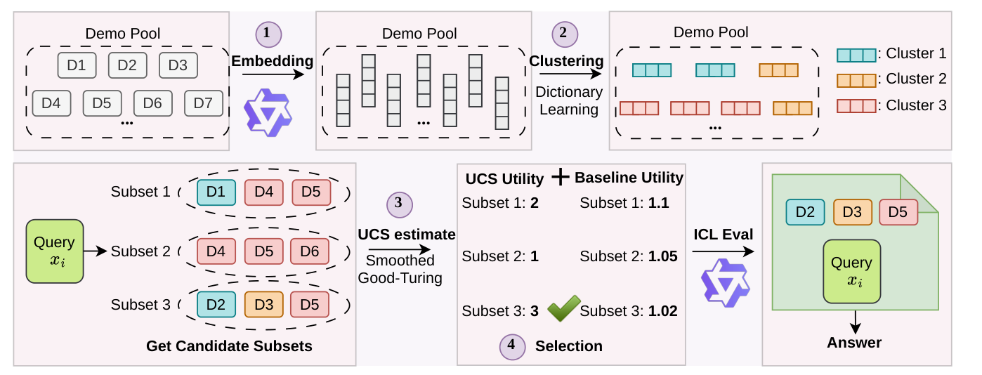
The coverage term can favor a set that spans more clusters even when its baseline utility is slightly lower.

Our qualitative audit on BANKING77 illustrates how this can change prompt content. With Qwen2.5-7B, we find clusters of identity-verification paraphrases and duplicate-charge queries. Adding UCS to DPP shifts selections toward smaller, more specific groups, including identity verification and ATM cash issues. These examples show that some induced clusters capture recognizable task patterns.

Results under the same prompt budget

In our intent-classification experiments, we compare selectors at a fixed budget of ten demonstrations, using 500 test examples and three runs per setting. The largest gains in these experiments occur with query-independent VoteK. With Qwen2.5-7B, UCS raises accuracy from 60.9% to 67.1% on HWU64 and from 70.3% to 74.4% on CLINC150.

Gains for query-dependent selectors are generally smaller. Llama-3.2-3B with MDL improves from 71.8% to 73.2% on BANKING77, while Gemma-2-9B with DPP remains at 99.0% on CLINC150.

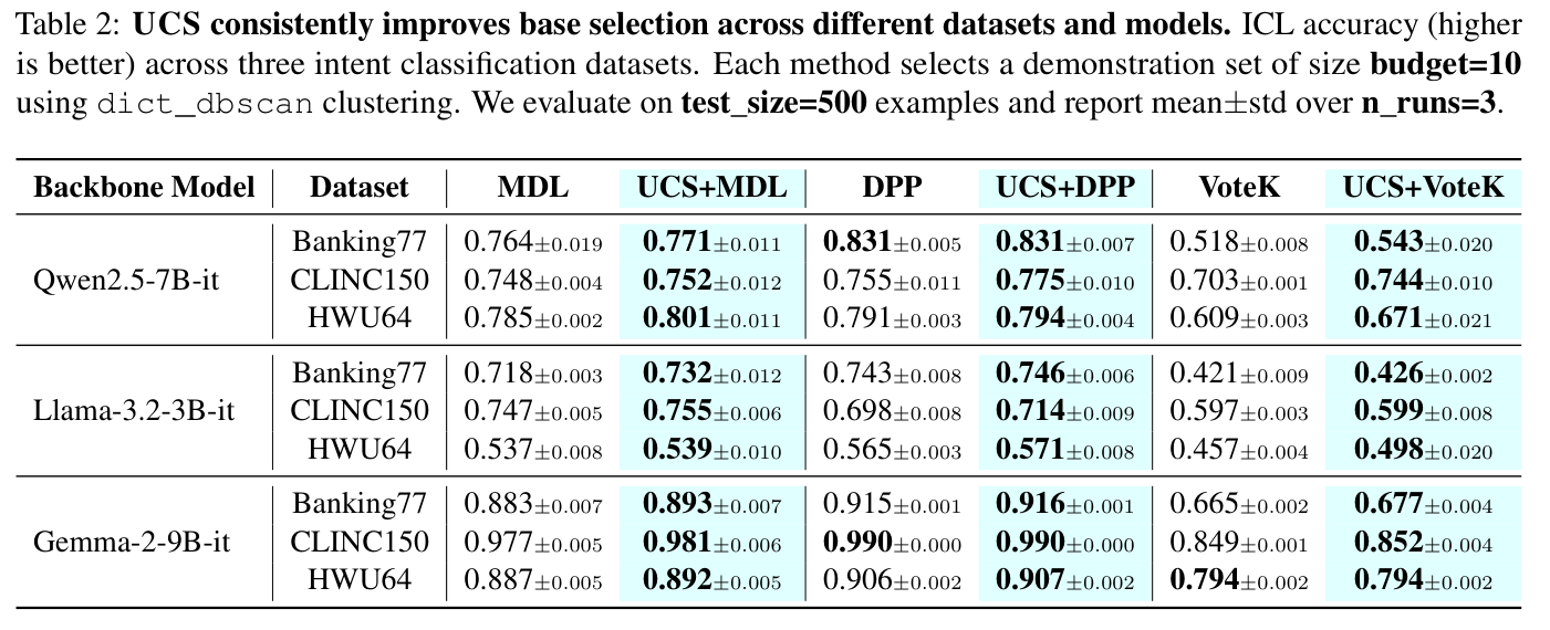
Adding coverage helps most in the VoteK settings; several stronger baselines change little. Values are mean ± standard deviation over three runs.

Our score ablation tests whether unseen estimation adds value beyond counting observed clusters. On HWU64 with Llama-3.2-3B and DPP, using only the observed count gives 54.3% accuracy, compared with 57.1% for the combined UCS score.

We also evaluate three BBEH reasoning tasks with Qwen2.5-7B. UCS improves eight of the nine selector–task combinations in Table 3, including 13.3% to 25.8% on Shuffled Objects with DPP; VoteK on that task remains at 24.2%. Each task has only 40 test examples, so these results provide initial evidence beyond intent classification.

Where the approach is limited

Embedding a large candidate pool with the model used for inference can be expensive. A practical goal is to estimate coverage with a cheaper model, select demonstrations using that signal, and pass the selected labelled examples to a more expensive target model. This requires the coverage signal to transfer across models.

Our cross-model experiment investigates whether models can share a coverage representation. We align embeddings from Qwen2.5-7B, Llama-3.2-3B, and Gemma-2-9B through orthogonal transformations and jointly learn a dictionary and codes. We then use the joint dictionary to construct UCS priors for DPP selection, evaluating the resulting prompts with Qwen or Llama. We use all three models’ embeddings in this experiment, so it does not itself eliminate the target model’s embedding cost.

The shared dictionary does not consistently improve selection. For Qwen, accuracy drops from 79.4% to 67.5% on HWU64 and from 83.1% to 78.3% on BANKING77, although it improves from 77.5% to 82.3% on CLINC150. Llama stays close to its single-model results.

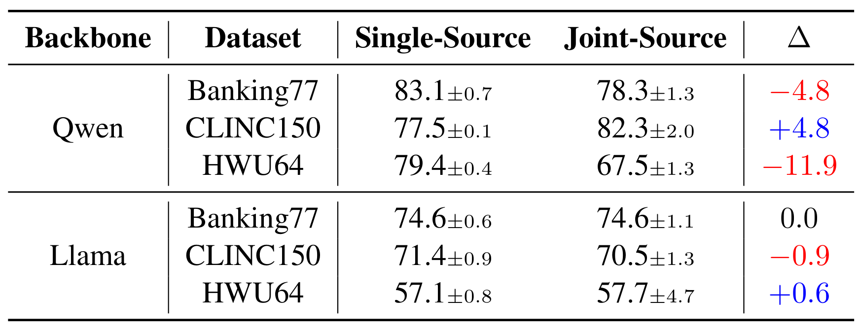
The joint dictionary gives mixed results at the same ten-demonstration budget. Its largest loss is 11.9 percentage points for Qwen on HWU64, while Llama changes relatively little.

As we discuss in Section 5.1, a shared linear space may blur useful model-specific distinctions. These mixed results support our default of constructing coverage in the inference model’s own representation space; reliable selection with a cheaper model’s coverage signal remains an open problem.

UCS also depends on the clusters it discovers, and unsupervised clusters need not align with human concepts. We tune clustering granularity and the coverage weight for the model, dataset, and selector (Appendix D). Most of our experiments use short intent-classification inputs. We leave longer contexts, generation-heavy tasks, and newer learned selectors for further study.

The computational cost depends strongly on the integration. In Appendix B, we report roughly 38–57 seconds of one-time preprocessing per dataset–model pair on an A100 80GB. The measured end-to-end time differences are −0.09 to +2.28 seconds for MDL and −13.37 to +2.75 seconds for VoteK. DPP adds roughly 606–681 seconds because it recomputes coverage inside its greedy loop. These are differences for complete evaluation runs, including selection and ICL inference.

Within these limits, UCS offers a way to make prompt composition more deliberate: retain the selector’s existing signals, then account for which patterns the set represents and which remain underexplored.

Reference

Jiayi Xin, Xiang Li, Evan Qiang, Weiqing He, Tianqi Shang, Weijie J. Su, and Qi Long. 2026. UCS: Estimating Unseen Coverage for Improved In-Context Learning. Findings of the Association for Computational Linguistics: ACL 2026, pp. 10965–10981. doi:10.18653/v1/2026.findings-acl.533.

The implementation is available in our official code repository.

Related reading

Evaluating the Unseen Capabilities: How Many Theorems Do LLMs Know?, by Xiang Li, Jiayi Xin, Qi Long, and Weijie J. Su, introduces KnowSum. It estimates unseen knowledge within a class of evaluation tasks by extrapolating from the frequencies of observed knowledge instances. UCS brings related statistical reasoning to demonstration selection: its units are clusters of candidate examples, and the estimate helps decide what to put in the prompt.

All research articles · Publications