Should rewording a question change its uncertainty?

Jiayi Xin

Topics: Large language models · Uncertainty quantification · Conformal prediction

Paper · Code

The answer stayed the same. The uncertainty moved.

Consider two questions: “What is the capital of France?” and “Which city serves as France’s capital?” The correct answer is unchanged. Ideally, an uncertainty estimate should also be similar. Yet a language model can assign noticeably different probabilities to the same answer options after this small rewrite. A downstream uncertainty procedure can then return a different set of plausible answers.

To see where that change comes from, start with conformal prediction. Each candidate answer receives a nonconformity score, with lower values indicating a better fit. A threshold learned from held-out calibration examples determines which answers enter the prediction set. Under exchangeability, the method guarantees at least the target marginal coverage. In the example below, only Paris is included.

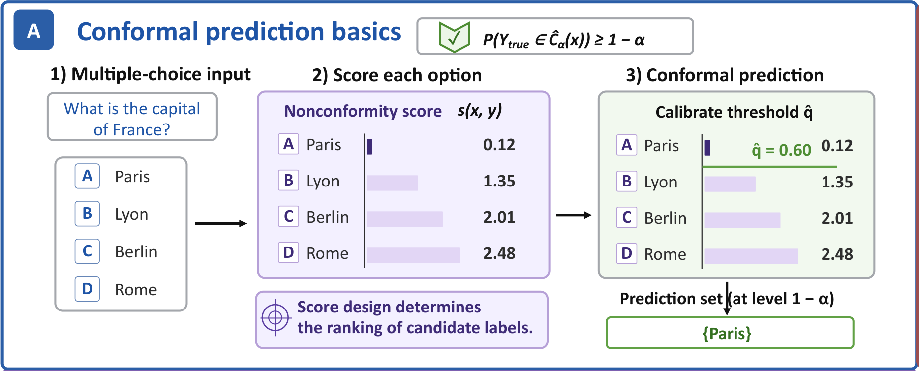
Figure 1A. A calibrated threshold selects Paris from the candidate answers in this schematic example.

That coverage guarantee does not by itself make uncertainty stable across equivalent questions. When the wording changes, the scores can move and the prediction set can change with them. The next example illustrates the problem: one formulation returns Paris alone, while the other also includes Lyon. Both sets contain the correct answer, but they express different levels of uncertainty about the same fact.

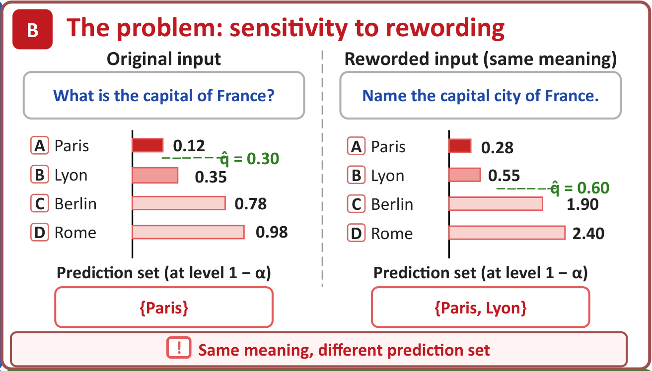
Figure 1B. Equivalent questions can lead to different prediction sets.

Our PA approach starts by giving the scoring procedure several views of the question. Whether the user supplies the original wording or a rewrite, PA generates its own internal paraphrases of that input. A frozen LLM produces a hidden representation for each view, and a lightweight learned proxy turns those representations into probabilities over the answer options.

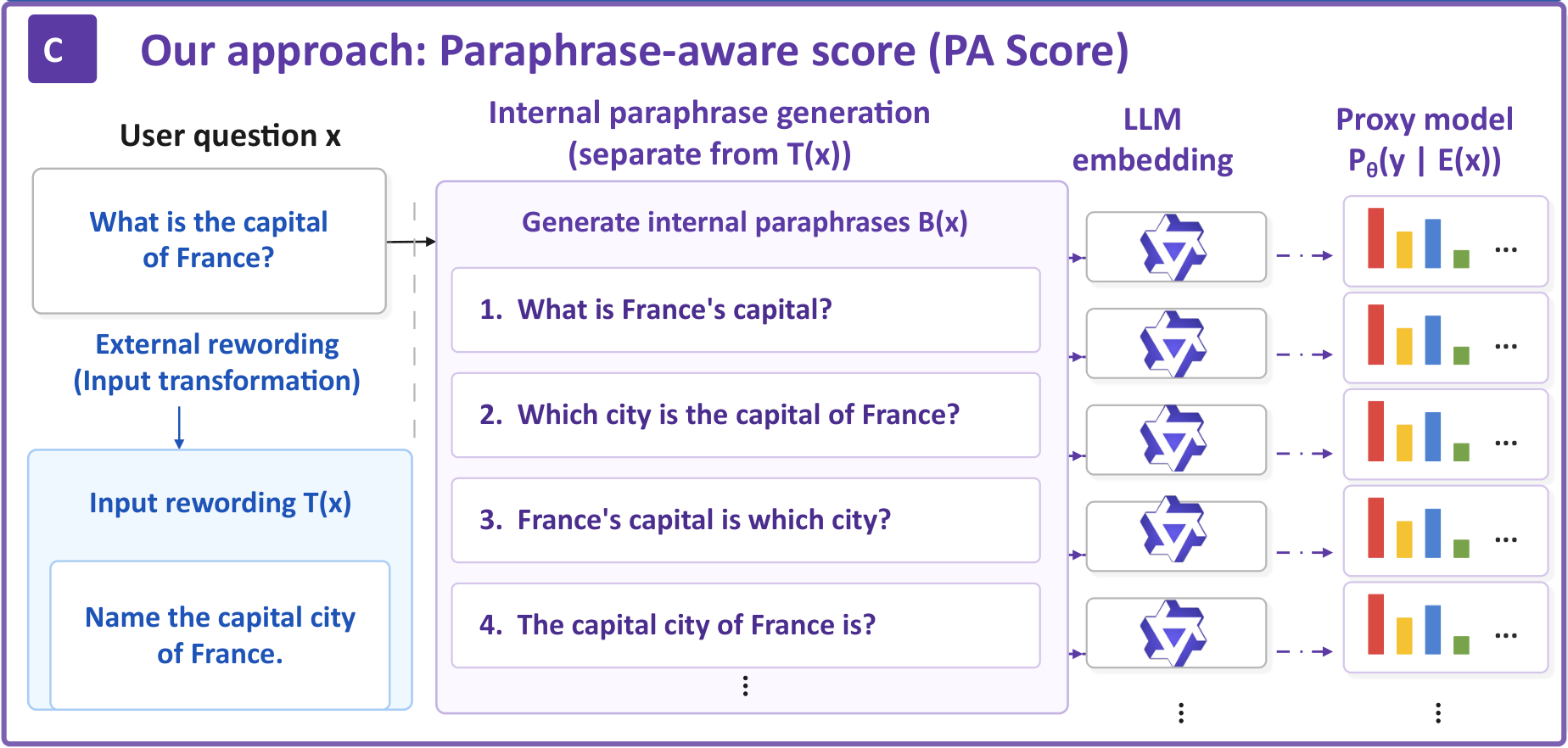
Figure 1C. PA generates internal paraphrases and scores each view with a learned proxy.

We then aggregate the per-paraphrase scores for each answer and calibrate the resulting PA score. The final example brings us back to the original goal: both formulations now produce the set containing Paris. Pooling evidence across paraphrases makes the score less dependent on a single wording. The conformal step still controls marginal coverage under its assumptions, while the score design shapes the set’s compactness and sensitivity to rewording.

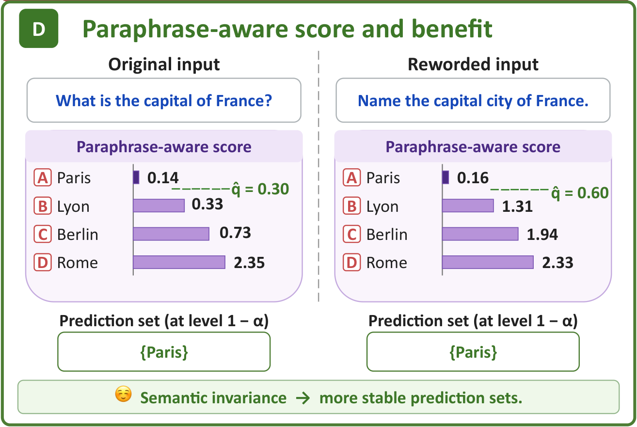
Figure 1D. Both wordings yield the same prediction set after paraphrase-aware scoring.

First, train a proxy that can score the answers

The training panel follows three familiar questions: the capital of France, the largest planet in the Solar System, and the author of 1984. Their labels are Paris, Jupiter, and George Orwell. Each question is expanded into paraphrases that keep its answer choices and correct label. For example, “Name the capital of France” becomes another training view with Paris as its target.

For each view, the frozen LLM reads the question and answer choices without seeing the correct label. We extract its final-layer hidden representation, denoted by $E(v)$ for a view $v$. A two-layer MLP with parameters $\theta$ maps this representation to a distribution $P_\theta(y\mid E(v))$ over candidate answers $y$. Training updates the small proxy while leaving the LLM fixed.

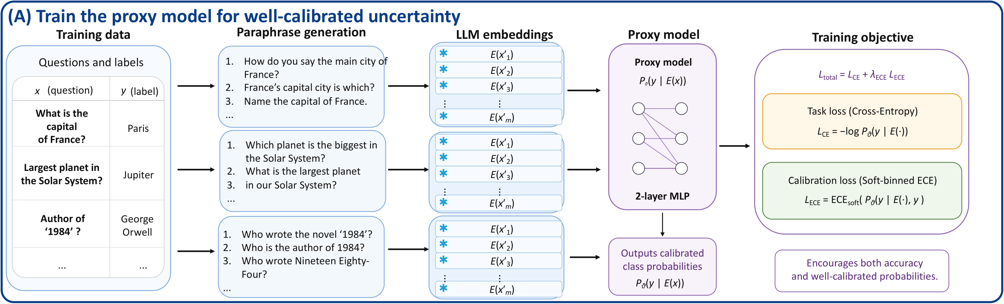
Figure 2A. Each paraphrase inherits the original answer label, giving the proxy several ways to learn the same question.

The training objective combines answer accuracy with probability calibration:

For a training view $v$ with correct answer $y$, the cross-entropy contribution is $-\log P_\theta(y\mid E(v))$. It rewards assigning probability to the correct answer. The soft-binned expected calibration error term, $\mathcal L_{\mathrm{ECE}}$, encourages confidence to agree with observed accuracy; $\lambda_{\mathrm{ECE}}$ controls its weight. Thus, the Paris examples teach the proxy both which answer to favor and how confidently to favor it.

Proxy training and conformal calibration serve different purposes and use separate data. In our main experiments, we divide each 10,000-question dataset 40/30/30 into training, calibration, and test splits. Of the 4,000 training questions, we reserve 600 for validation. We fix the proxy and its hyperparameters before using the held-out calibration labels to choose prediction-set thresholds, as detailed in Appendix D.

Then, combine the views of a new question

At inference, the answer is unknown. PA generates internal paraphrases of the arriving question, embeds them with the same frozen LLM, and runs the trained proxy on each representation. The France example gives several probability estimates for Paris, several for Lyon, and so on. We combine the estimates separately for each candidate answer, so the final set can still contain more than one option.

Figure 2B. PA combines evidence across paraphrases for each answer before deciding which answers belong in the set.

Write $x$ for the input currently being scored, which may already be an external rewrite, and let $B(x)={x’_1,\ldots,x’_m}$ be its $m$ internal paraphrases. For candidate answer $y$, the base score from view $j$ is

A likely answer has a low score. We study three ways to turn these per-view scores into one label-wise PA score.

The mean score gives every paraphrase equal weight:

For Paris, this averages its lack of support across the different formulations. One unusually difficult wording contributes to the result without determining it alone.

The distance-weighted score gives more weight to paraphrases whose hidden representations are close to that of the arriving input:

Here $\lVert\cdot\rVert_2$ is Euclidean distance. A smaller distance gives a larger positive weight, so nearby views contribute more. This version uses the arriving question as an embedding anchor as well as using its internal paraphrases.

The worst-case score takes the largest nonconformity score across the views:

Paris receives a low worst-case score only if every generated view gives it strong support. This emphasizes difficult paraphrases, but it also makes the score sensitive to a poor rewrite. We give these three definitions in Section 4 and Table 1.

Calibrate the complete scoring rule

Before deployment, we run the chosen scoring procedure on held-out calibration questions and record the score of each known correct answer. For $n$ calibration examples and target coverage $1-\alpha$, split conformal prediction uses the $\lceil(n+1)(1-\alpha)\rceil$-th ordered score as its threshold $\hat q$, taking $\hat q=\infty$ if that index is $n+1$. Each score variant gets its own threshold because changing the aggregation changes the score distribution.

For a new question, the prediction set is

In the France example, Paris is retained when its aggregated score lies below the calibrated threshold; each distractor is checked in the same way. The threshold is already fixed, so the test answer is never needed to construct the set. In our experiments, we replace an empty thresholded set with the most probable label. We also evaluate quasi-conditional conformal prediction, which adapts thresholds using features that group semantically related questions.

When does coverage survive rewording?

Our evaluation separates changes in wording from a mismatch between calibration and deployment. In the normal setting, calibration and test questions keep their original wording. In the fully reworded setting, both are externally rewritten. In the semi-reworded setting, calibration questions stay original while only test questions are rewritten. PA still generates its own internal paraphrases in all three settings.

Table 2. Test-only rewording needs an additional alignment condition because calibration and deployment receive differently transformed inputs.

Assume the original examples are independent draws from the same distribution, and hold the learned proxy and scoring rule fixed. Normal evaluation applies the same scoring pipeline to calibration and test examples. Fully reworded evaluation also treats both sides alike, using independently sampled rewrites from the same transformation. This preserves the score exchangeability required by split conformal prediction.

Semi-reworded evaluation is harder. A calibration question $x$ is scored through $B(x)$, while its reworded counterpart would be scored through $B(T(x))$. To align these score distributions, our analysis assumes distributional closedness. If $T(\cdot\mid x)$ denotes the paraphrase distribution, then

For the running example, generating internal views from “Name the capital city of France” must follow the same distribution as generating them from “What is the capital of France?” Merely preserving the correct answer does not establish that equality. Under this condition, independently sampled internal views restore score exchangeability for the mean and worst-case scores, giving the usual marginal coverage guarantee. The anchor-dependent weighted score needs alignment of the anchor and views jointly; QCCP additionally requires its joint feature–score assumptions. Appendix C gives the precise statements.

In the separate fixed-cutoff diagnostic in Appendix E.4, we keep the clean-trained proxy and clean calibration threshold unchanged while rewriting the same test questions. With Qwen3-8B, mean PA scoring, and split conformal prediction, coverage after rewriting averages 85.5% on MMLU and 87.6% on HaluDial over three seeds, below the 90% target reported in Table 15.

What changes in the experiments?

We evaluate seven multiple-choice benchmarks with six answer options and a 90% target coverage. The five general-domain datasets in the main table are MMLU (QA), CosmosQA (RC), HellaSwag (CI), and the dialogue and summarization subsets of HaluEval, called HaluDial (DRS) and HaluSum (DS). Two further datasets test medical QA. We convert these tasks to a shared six-option format that includes “I don’t know” and “None of the above.”

The main comparison below uses Qwen3-8B. Read coverage and set size together: a set containing every option can cover the answer without being very informative. On fully reworded HaluDial under split conformal prediction, PA returns an average of 1.36 answers, compared with 3.37 for our label-wise TRON adaptation. Empirical coverage is 90.40% and 91.53%, respectively. The same table shows how that trade-off varies across datasets and the two conformal frameworks.

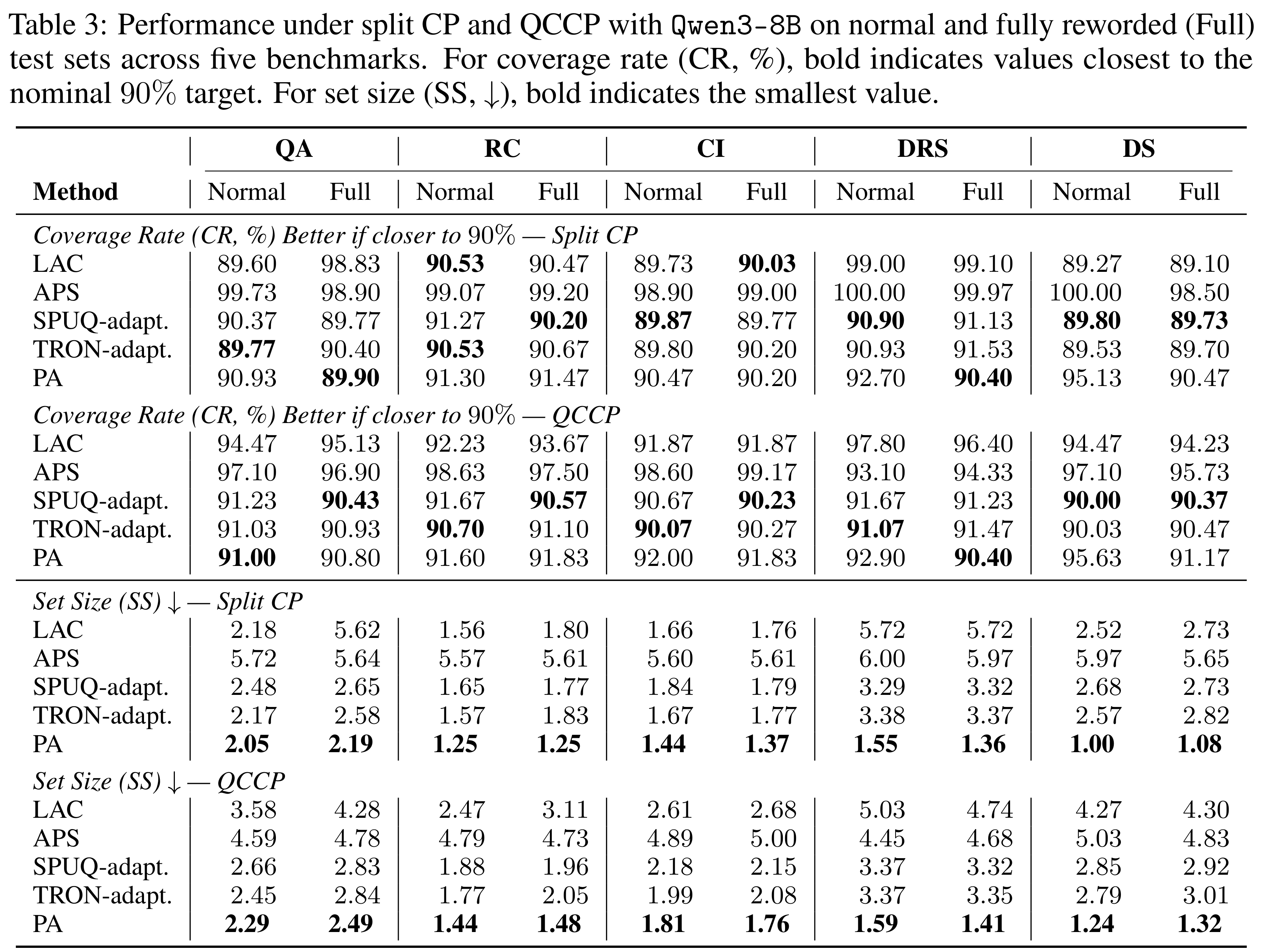
Table 3. PA produces the smallest sets in these comparisons, with achieved coverage reported alongside each result.

Why the proxy matters

The proxy improves the quality of the probabilities that enter the score. In Figure 3, its accuracy is higher and its Brier score and negative log-likelihood are lower across the five tasks. Brier score measures squared error between the predicted probability vector and the correct one-hot label; negative log-likelihood penalizes low probability on the correct answer. Together, they show whether the distribution is useful beyond its top prediction.

For example, HaluDial accuracy rises from 51.0% to 74.2%. On CosmosQA, Brier score falls from 0.075 to 0.039 and negative log-likelihood from 2.513 to 0.487. These are improvements from the learned proxy, so they help explain why much of PA’s compactness gain appears before inference-time aggregation is added.

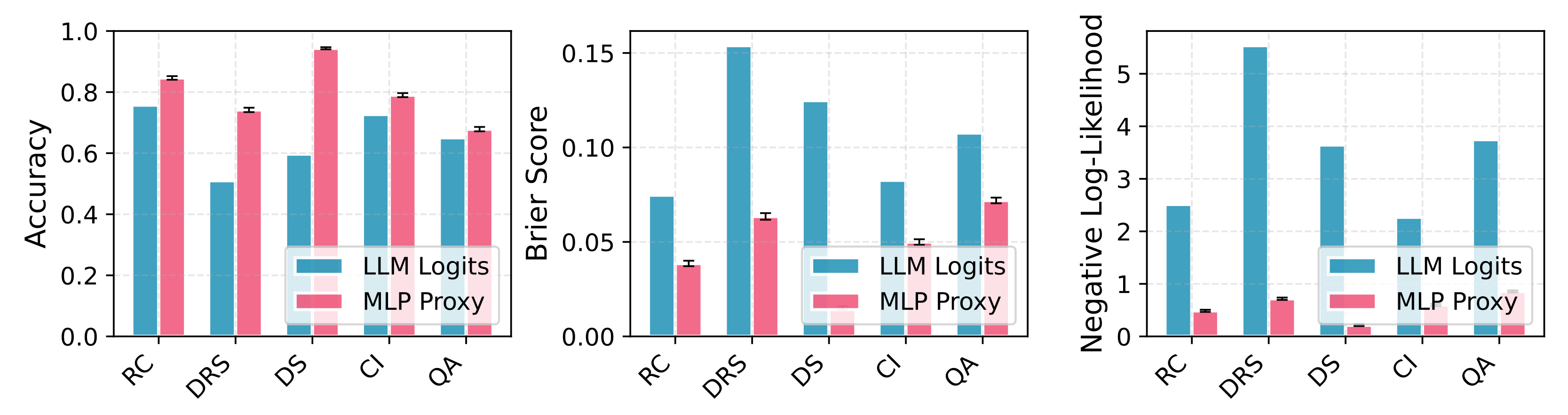
Figure 3. The proxy improves both answer selection and the probability distribution used for scoring.

Our controlled ablation makes that attribution explicit. Averaged over five datasets and three seeds, a hidden-state proxy trained only on original questions reduces semi-reworded set size from 2.8929 to 1.3725. It accounts for most of the reduction before paraphrase training or multi-view inference is introduced.

Holding a paraphrase-augmented proxy checkpoint fixed, six-view scoring then reduces the average number of labels that enter or leave the prediction set after a rewrite from 0.2029 to 0.1708, a 15.8% reduction. Coverage changes from 89.96% to 89.81%, and average set size from 1.3587 to 1.3331. Simply averaging raw LLM probabilities increases set changes in the same ablation. The proxy and aggregation therefore contribute different benefits: more informative scoring and additional wording stability.

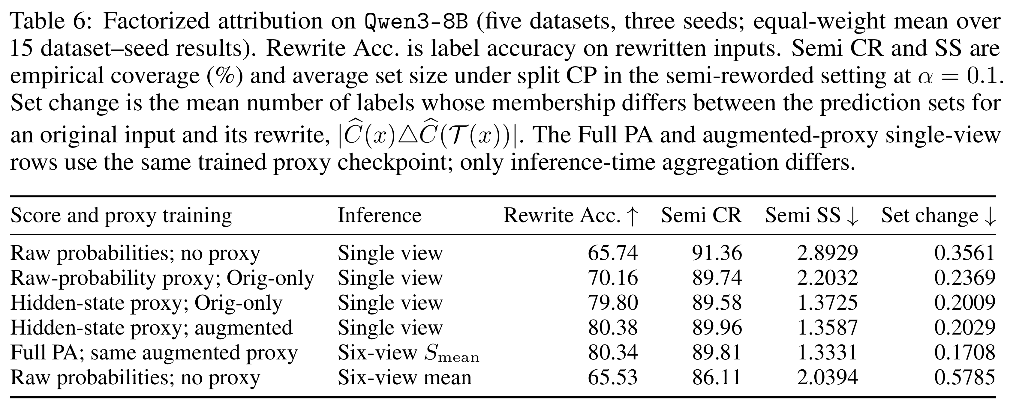
Table 6. Comparing the same augmented proxy with one or six views isolates the effect of inference-time aggregation.

Which aggregation is useful?

In Figure 6, we compare the three score variants across seven datasets under QCCP. Mean and distance-weighted aggregation behave similarly, producing average set sizes around 1.9–2.0. Worst-case aggregation produces somewhat larger sets, around 2.0–2.2, and is more conservative in the semi-reworded setting: its average coverage is 93.0%, compared with 90.1% for mean and 90.6% for weighted scoring. The extra emphasis on difficult views therefore has a visible coverage–size trade-off.

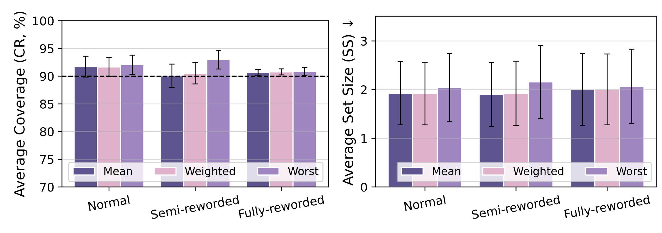
Figure 6. Emphasizing the hardest paraphrase adds conservatism, while mean and weighted aggregation give similar results here.

How far does the evidence extend?

Our main evidence comes from English multiple-choice QA, but in Appendix G.3, we also include a preliminary FEVER claim-verification experiment. We treat an atomic claim as a binary True/False problem, generate paraphrases, and apply the same proxy-and-aggregation pipeline. With Qwen3-8B, fully reworded PA reaches 90.5% coverage under split CP and 90.3% under QCCP, with an average set size of 1.000 in both. Since the LAC baseline also produces essentially singleton sets, this experiment primarily examines coverage after rewording rather than a large reduction in set size.

That result is a first step toward factuality assessment at the claim level. Applying it to a long generated answer would additionally require extracting its claims and combining claim-level results into a response-level guarantee. Those steps remain future work.

In Appendix G.4, we propose an extension to images. For visual question answering, we suggest constructing image variants with small Gaussian perturbations that preserve the relevant content, extracting answer-token hidden representations from a frozen vision–language model, and aggregating scores over the variants. We haven’t yet explored image inputs experimentally, but we see this as a promising direction for future work. We’d be excited to see how paraphrase-aware scoring extends to visual question answering and other multimodal tasks.

The cost of extra views

Our strongest PA variant needs labeled proxy-training data and access to hidden states. We also tested an API-only extension, but it does not match the white-box version. Paraphrase quality matters too: semantic drift changes the task, while insufficient diversity limits what the extra views contribute. Our coverage analysis addresses the stated rewording conditions, leaving shifts such as changing topics or factual knowledge outside its scope.

Online generation is a substantial practical cost. In our timing experiments with Qwen3-8B on one NVIDIA B200, the full six-view pipeline is 22.7–83.4 times slower than raw single-input inference, with paraphrase generation accounting for 67–97% of the time. The cached scoring measurement is much smaller, at most 0.20 ms per question, but assumes both the paraphrases and their hidden representations have already been computed. It measures the remaining proxy, aggregation, and set-construction work, as specified in Appendix E.6.

PA makes a question’s semantic neighborhood part of its uncertainty score. Our results show why both parts matter: learning a better scorer makes the sets more informative, and combining its judgments across paraphrases makes them more stable. The remaining challenge is to retain those benefits when the task, available representations, or cost of generating views changes.

Reference

Jiayi Xin, Evan Qiang, Zihan Zhu, Xiang Li, Weijie J. Su, and Qi Long. 2026. Conformal Prediction with Paraphrase-Aware Scoring for LLM Uncertainty Quantification. arXiv:2610.04239. NeurIPS 2026 poster.

All research articles · Publications